Introduction
It has been a while since I posted articles about GAN and WGAN. I want to close this series of posts on GAN with this post presenting gluon code for GAN using MNIST.
GAN is notorious for its instability when train the model. There are two main streams of research to address this issue: one is to figure out an optimal architecture for stable learning and the other is to fix loss function, which is considered as one of the primary reasons for instability. WGAN belongs to the latter group defining a new loss function based on a different distance measure between two distributions, called Wasserstein distance. Before, in original vanilla GAN paper, it was proven that adversarial set of loss functions is equivalent to Jenson-Shannon distance at optimal point. For more detailed information about GAN, please refer to Introduction to WGAN
Wasserstein distance
A crucial disadvantage of KL(Kullback - Leibler) divergence based metric(Jenson - Shannon distance is just an extention of KL distance to more than two distributions) is that it can be defined only for the distributions that share the same support. If it is not the case, those metrics explodes or be a constant so that they cannot represent the right distance between distributions. WGAN paper has a nice illustration on this and if you need more detailed explanation, you can read this post.
This problem was not a big problem in classification tasks since, entropy-based metric for categorical response has limited number of categories and ground-truth distribution and its estimator must share the support. It is totally different story for generation problem since we need to generate a small manifold in a huge original data space. Needlessly to say, it must be very hard for a set of tiny manifolds to share their support. Let’s think about MNIST. Assuming gray image, images dwell in $255^{784}$ dimensional space but the size of collected data at hand is 60,000. I cannot tell precisely but meaningful images that look like hand-written numbers are rare in the entire space of 28 $\times$ 28 sized images.
Wasserstein distance can measure how much distributions are apart even when those distributions do not share supports. It is very good thing but calculating Wasserstein distance is not easy to get since it involves another optimization problem itself. Kantorvich-Rubinstein duality tweaks the original optimization problem into a much simpler maximization problem under a certain constraint. The main idea of WGAN is that neural network can be used for finding accurate Wasserstein distance. Here is a formal definition of Wasserstein distance.
To get more sense, I just depicted what the above equation means at below.
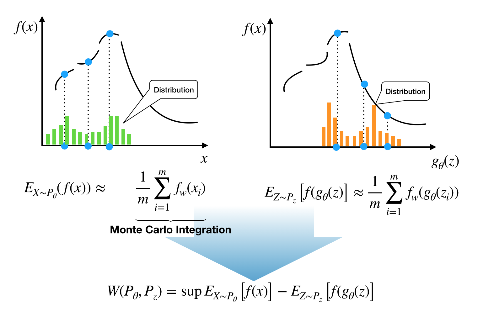
The function $f$ in the above figure is just an example. What we will going to do is to search the function that maximizes expection amongst all possible $K$ - Lipschitz functions. It must be very extensive work and the authors of WGAN suggested let neural network takes care of it.
In a sense that WGAN tells us a real numbered distance between real and generated data’s distribution, WGAN can be thought of as a more flexible version of GAN that just say yes or no for the question “Are two distributions the same?”.
Critic vs Discriminator
WGAN introduces a new concept critic, which corresponds to discriminator in GAN. As is briefly mentioned above, the discriminator in GAN only tells if incoming dataset is fake or real and it evolves as epoch goes to increase accuracy in making such a series of decisions. In contrast, critic in WGAN tries to measure Wasserstein distance better by simulating Lipschitz function more tightly to get more accurate distance. Simulation is done by updating critic network under implicit constraint that critic network satisfies Lipschitz continuity condition.
If you look at the final algorithm, they, GAN and WGAN, look very similar to each other in algorithmic point of view, but their derivation and role is quite different as much as variational auto encoder is different from autoencoder. One fascinating thing is that the derived loss function is even simpler than the loss function from the original GAN algorithm. It’s just difference between two averages. The following equation is taken from the algorithm in the original WGAN paper.

Critic implementation
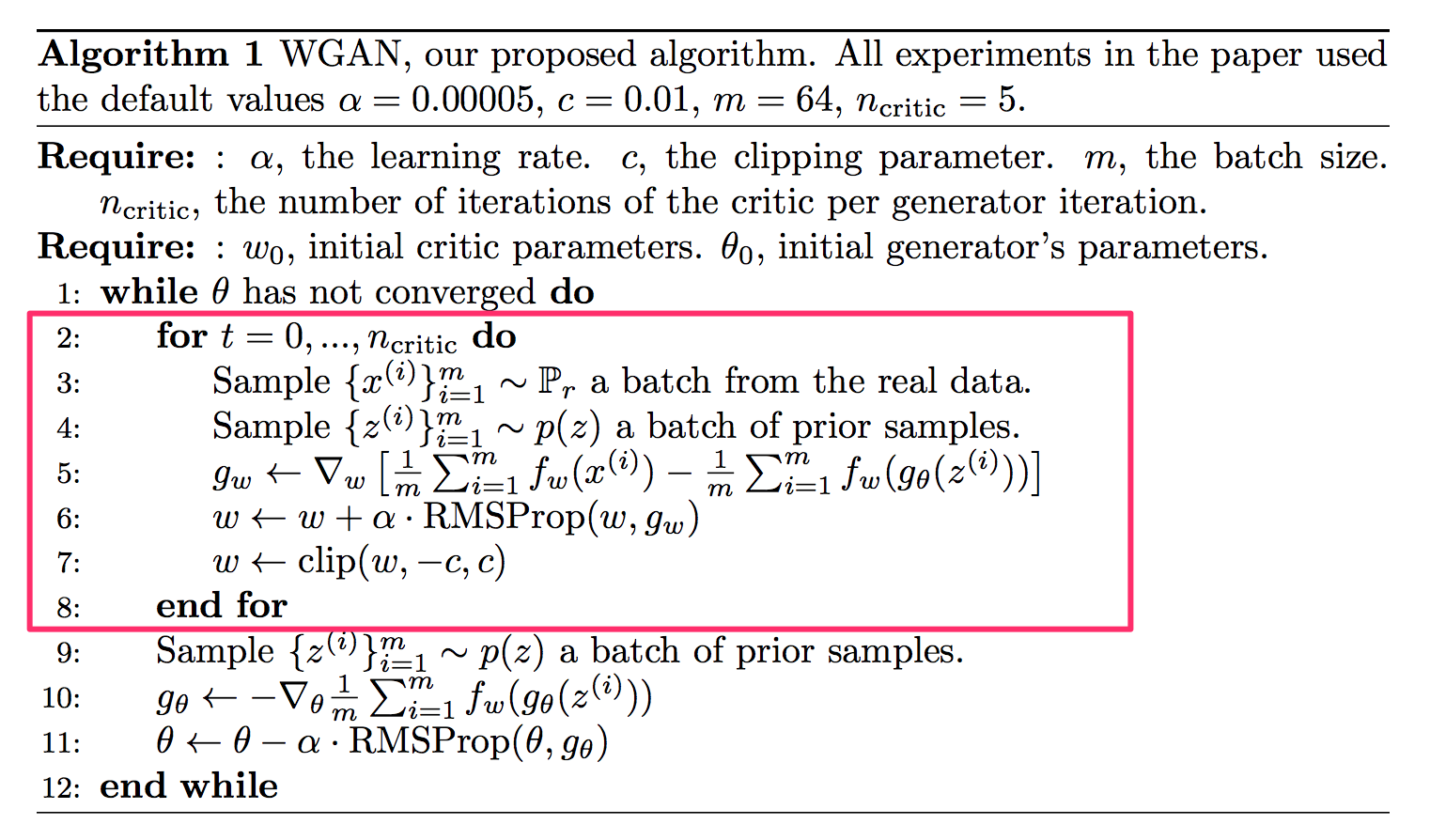
The entire algorithm is given below. Especially critic implmentation is highlighed with pink box. When a set of data is given, the algorithm first compares with a set of generated images. To get more accurate distance, it iterates through several steps for critic network to end up with the maximum difference of expectations from real and fake data, which is wasserstein distance. It my fail to find exact distance, but we want to be as close as possible.
The relevant part of the implementation looks like this. (It’s gluon)
for j in range(n_critic_steps):
    latent_z = nd.random.normal(shape =(batch_size, latent_dim), ctx = ctx) # Latent data
    fake_data = gen(latent_z)
    c_real = nd.mean(critic(real_data))
    c_fake = nd.mean(critic(fake_data))
    with autograd.record():
        c_cost = - (c_real - c_fake)
        c_cost.backward()
    critic_trainer.step(batch_size)
    # Weight clipping
    [critic.collect_params()[p].set_data(nd.clip(critic.collect_params()[p].data(), -clip, clip)) for p in critic.collect_params()]
According to the definition of Wasserstein distance, we need to maximize the expectations under two different distributions. For utilizing built-in optimizers in Gluon, we defined cost as negative of the value we want to maximize.
At the end of each critic update steps, to make sure that a function, the critic network surrogates, satisfies Lipschitz continuity condition, the weights are clipped not to let critic network violate Lipschitz condition. The authors didn’t like this heuristic approach though.
Since the first part of Wasserstein distance does not involve generator network’s parameter $\theta$, we can ignore the first part of Wasserstein distance.
Only considering the latter part, we can update the generator network as follows:
latent_z = nd.random.normal(shape = (batch_size, latent_dim), ctx =ctx)
with autograd.record():
    fake = gen(latent_z)
    g = nd.mean(critic(fake))
    g_cost = - g
    g_cost.backward()
gen_trainer.step(batch_size)
The entire code can be found in git repository
Penalization
In the original WGAN, the Lipschitz constraint was exposed using weight clipping and there was an obvious room for improvement. Instead, the authors in Improved Training of Wasserstein GANs proposed to expose penalty on the norm of weights from critic network. It is one of natural way to control the magnitude of weight matrix to make critic network satisfies Lipschitz condition. The following code shows “penalty part” from the entire implementation.
def get_penalty(critic, real_data, fake_data, _lambda):
    from mxnet import autograd
    alpha = nd.random.uniform(shape = (batch_size,1))
    alpha = nd.repeat(alpha, repeats = real_data.shape[1], axis = 1)
    alpha = alpha.as_in_context(mx.gpu())

    interpolates = alpha * real_data + ((1 - alpha) * fake_data)
    interpolates.attach_grad()
    with autograd.record():
        z = critic(interpolates)
    z.backward()

    gradients = interpolates.grad
    gradient_penalty = nd.mean(nd.array([(x.norm()**2 - 1).asscalar() for x in gradients], ctx = ctx)) * _lambda

    return gradient_penalty
The rest of the algorithm is exactly the same as that of WGAN.
Results and thoughts
After 400 epochs, I just printed the generated image. Even after 400 epochs, I could not get perfact hand-written number images yet.
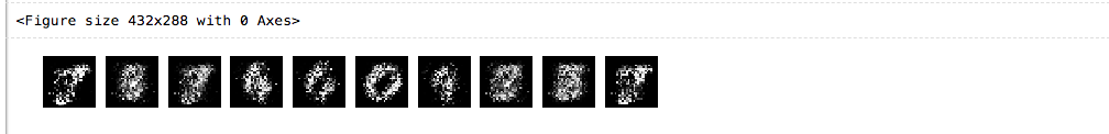
According to my experience, those two algorithms seem to be comparable. My personal feeling is that it’s still very hard to generate an images even with WGAN and improved WGAN.