Introduction

There are many methods for sentence representation. We have discussed 5 different ways of sentence representation based on token representation. Let’s briefly summarize what is dealt with in the previous posts.

What we have discussed so far…

Just averaging token embeddings in sentence works pretty well on text classification problem. Text classification problem, which is relatively easy and simple task, does not need to understand the meaning of the sentence in semantic way but it suffices to count the word. For example, for sentiment analysis, the algorithm needs to count word that has siginificant relationship with positive or negative sentiments regardless of its position and meaning. Of course the algorithm should be able to learn the sentiment of word itself.

RNN

For better understanding of sentence, the order of words should be considered more importantly. For this, RNN can extracts information from a series of input tokens at hidden states as below:

$H = (h_1, \ldots, h_T), \quad h_i \in \mathbb R^d$

When we use those information, we frequently use the hidden state at the last time step only. It is not so easy to express all information from the sentence stored at only a small sized vector.

CNN

Borrowing the idea from $n$-gram techniques, CNN summarize local information around the token of interest. For this we can apply 1D convolution as is depicted in the following figure. This is just an example and we can try other different architecture too.

1d_conv_1

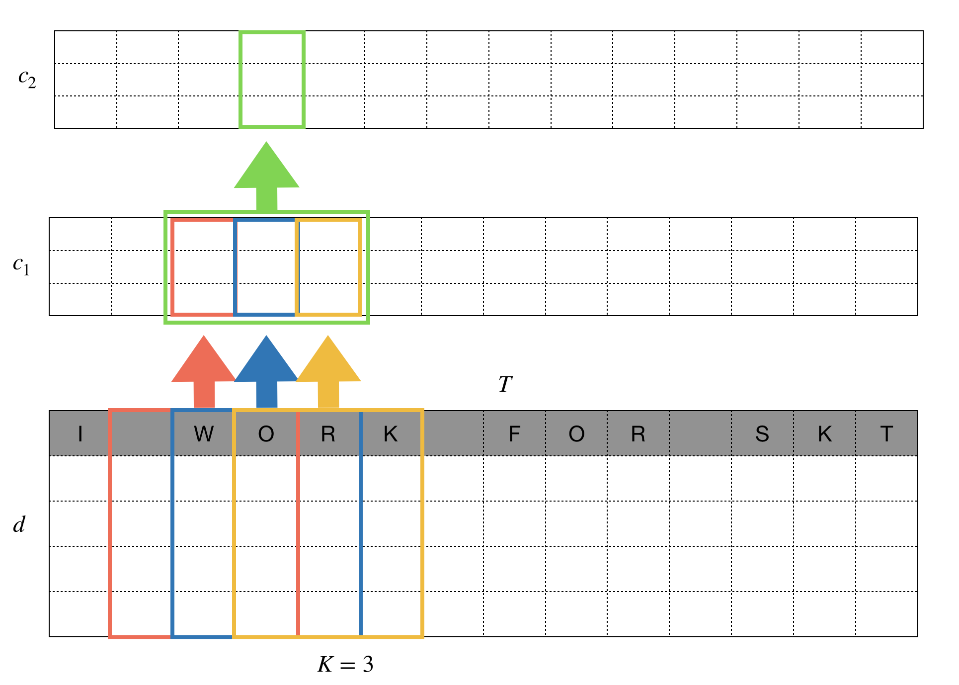
1D kernel of size 3 scan the tokens around the position we want to summarize information for. For this, we have to use padding of size 1 to keep the length of the feature map after filtering the same as the original length $T$. The number of output channel is $c_1$, by the way.

Another fiter is be applied to the feature map and the input is finally transformed into $c_2 \times T$. This series of process mimics the way human read the sentence, by understanding meaning of 3 tokens and then combine them to understand higher level concepts. As a side product, we can enjoy much faster computation using well-optimized CNN algorithms implemented in deep learning frameworks.

Relation network

The pair of words may give us more clear information about the sentence. There are many cases where a word may have different meaning depending on the usage. for example, the word ‘like’ in ‘I like’ is different from that in ‘like this’. If we consider ‘I’ and ‘like’ together, we can be more clear about the sentiment of sentence then the case where we use ‘like’ and ‘this’ together. It is definitely positive signal. Skip gram is a technique to retrieve infromation from the pair of words. It does not have to be adjacent pairs. It allow the gap between them as the word ‘skip’ suggests.

rel_net

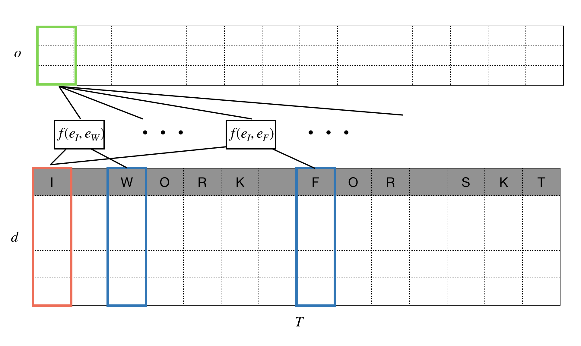
As you can see from the above figure, a pair of tokens are fed into a function $f(\cdot)$ to extract the relation between them. For a fixed position, $t$, the $T-1$ pairs are summarized, via sum or average or through any other relavant techeniques, for sentence representation.

A need for compromise

We can write down those three different approaches in a single general form as below:

$h_t = I_{t, 1}f(x_t, x_{1}) + \cdots + I_{t, (t-1)}f(x_t, x_{t-1}) + I_{t, (t+1)}f(x_t, x_{t+1}) + \cdots + I_{t, T}f(x_t, x_{T})$

With all $I_{t\cdot}$’s being 1, the general form says that any skip bigrams evenly contribute to the model.

In the case of RNN, we ignore any information after the token $x_t$, so the above equation reduces to

$h_t = f(x_t, x_{t-k}) + \cdots + f(x_t, x_{t-1}).$

With bidirectional rnn, we can consider backward relation from $x_T$ to $x_t$ though.

On the other hand, CNN browse information only around the token of interest, if we only cares about $k$ tokens before and after token $x_t$, the general formula can be re-arranged as below:

$h_t = f(x_t, x_{t-k}) + \cdots + f(x_t, x_{t-1}) + f(x_t, x_{t+1}) + \cdots + f(x_t, x_{t+ k})$

While relation network can be too big to consider all pairwise relationship of tokens, CNN can be too small to consider only local relationship between them. We need a compromise in between those two extreme, which is so called attention mechanism.

Self-Attention

A general form given in the previous paragraph can be re-written in a more flexible form as follows:

$h_t = \sum_{t' = 1}^T \alpha(x_t, x_{t'}) f(x_t, x_{t'})$

Here, $\alpha(\cdot,\cdot)$ controls the amount of effect that each pairwise combination of tokens may have. For example, two tokens, ‘I’ and ‘you’, in the sentence ‘I like you like this’, may not contribute to the decision on its sentiment. Contrarily, ‘I’ and ‘like’ combination gives us a clear idea about the sentiment of the sentence. In this case we pay little attention to the former and significant attention to the latter. By introducing the weight vector $\alpha(\cdot, \cdot)$, we can let the algorithm to adjust the importance of the word combination.

sa_mechanism

Supposing that $T$ tokens in the $i$-th sentence are embedded in $H_{i1}, \ldots, H_{iT}$, each token embedding will be assigned to a weight $\alpha_{it}$, which represents relative importance when tokens are summarized into a single representation. For this attention vector to address relative importance of word combinations, the attention weights must satisfy

$\sum_{t = 1} ^T \alpha_{i, t} = 1$

and this property is achieved by inserting soft-max layer as a node in the network.

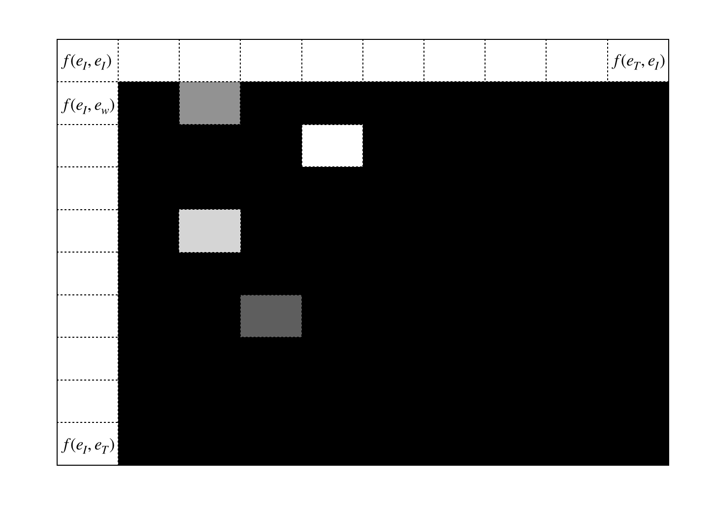
The final product we want to have at the end of the day is a weight matrix per input sentence. If we have 10 sentence feed into network, we will get 10 attention matrices that look like this.

sa_1

Self-Attention implementation

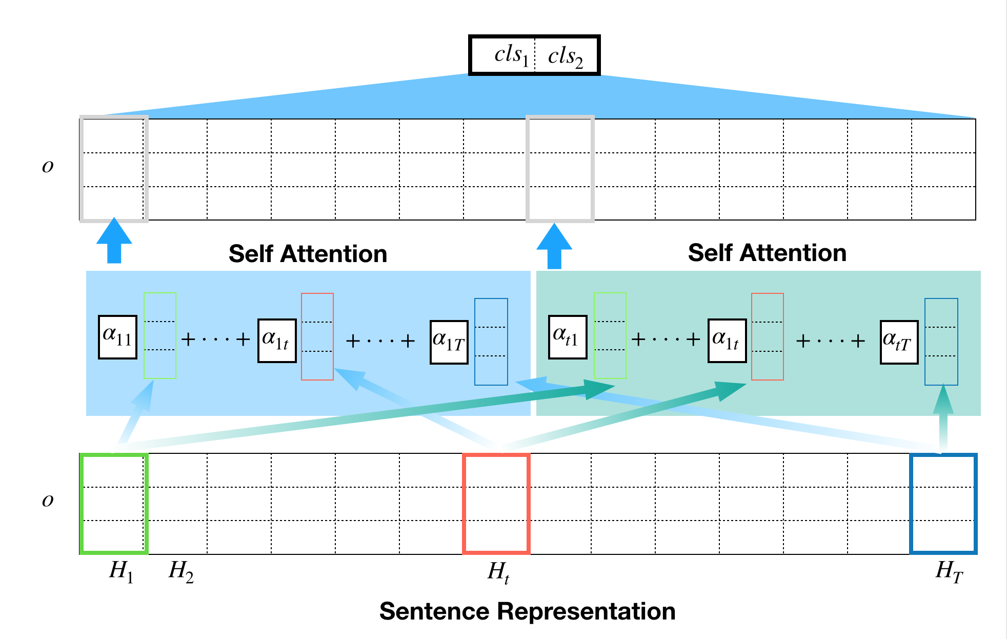
The self-attention mechanism was first proposed in the paper, A structured Self-Attentive Sentence Embedding, which applied self-attention mechanism to the hidden layer of bidirectional LSTM as shown in the following figure.

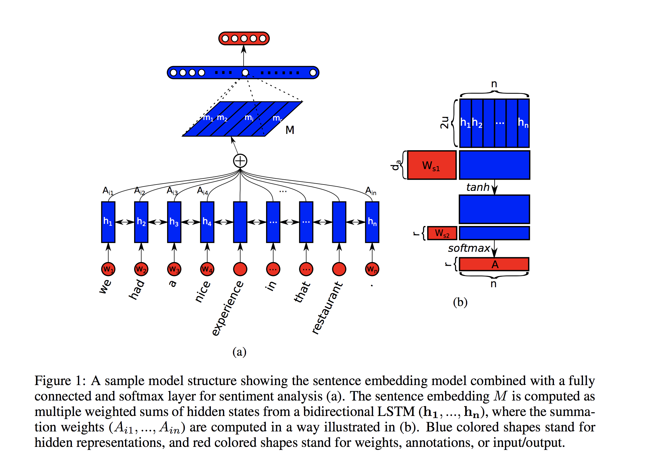
Structured Self-Attentive Sentence Embedding

It, however, does not have to be LSTM for token representation (not really token representation, what I mean by this is pre-sentence representation stage) and we will apply self-attention mechanism to token representation based on relation network.

Different from Self-attention mechanism from the original paper (given in the above figure, mathemtical details can be found in my previous post, here), attention mechanism for relation network can be defined as

sa_rel_net

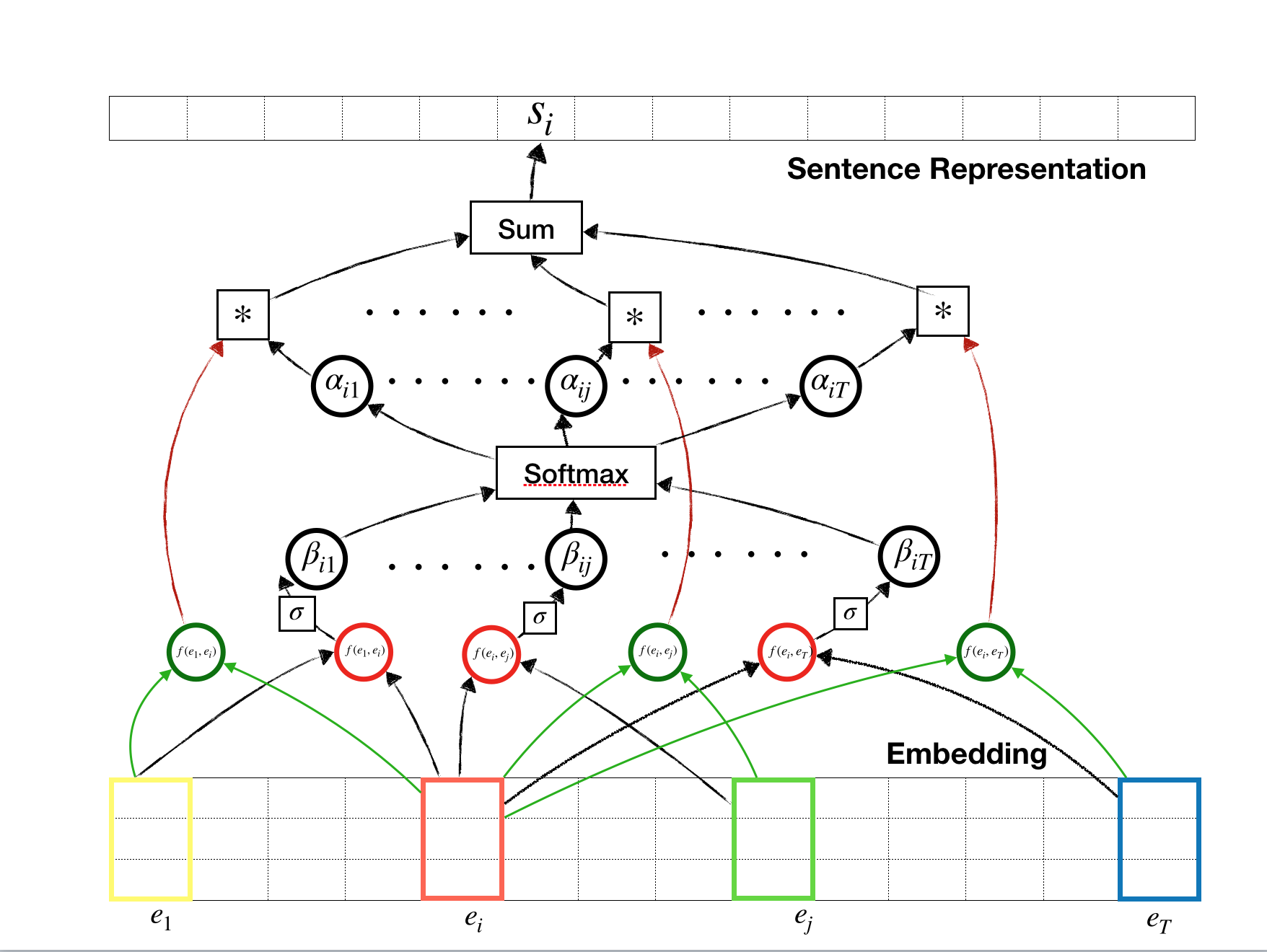
To explain the above diagram, let’s assume that we want to get a representation for the $i$-th token. For combinations of tokens with the $i$-th token, there are two outputs are produced: one of them is used for feature extraction (green circle) and the other is used for attention weight(red circle). Those two outputs may share the network, but in this article, we use separate network for each output. The output for the attnetion (red circle) runs through sigmoid and softmax layer before we get the final attention weights. These attention weights are multiplied to the extracted features to get the representation for a token of interest.

Self-Attention with Gluon

For the implementation, we assume very simple network with two fully connected dense layers for relation extractor and one dense layer for attention, which is followed by another two fully connected dense layeyrs for the classifier. Here, relation extractor and attention extractor is given the following code snippet.

class Sentence_Representation(nn.Block):
    def __init__(self, **kwargs):
        super(Sentence_Representation, self).__init__()
        for (k, v) in kwargs.items():
            setattr(self, k, v)
        
        with self.name_scope():
            self.embed = nn.Embedding(self.vocab_size, self.emb_dim)
            self.g_fc1 = nn.Dense(self.hidden_dim,activation='relu')
            self.g_fc2 = nn.Dense(self.hidden_dim,activation='relu')
            self.attn = nn.Dense(1, activation = 'tanh')
            
    def forward(self, x):
        embeds = self.embed(x) # batch * time step * embedding
        x_i = embeds.expand_dims(1)
        x_i = nd.repeat(x_i,repeats= self.sentence_length, axis=1) # batch * time step * time step * embedding
        x_j = embeds.expand_dims(2)
        x_j = nd.repeat(x_j,repeats= self.sentence_length, axis=2) # batch * time step * time step * embedding
        x_full = nd.concat(x_i,x_j,dim=3) # batch * time step * time step * (2 * embedding)
        # New input data
        _x = x_full.reshape((-1, 2 * self.emb_dim))
        
        # Network for attention
        _attn = self.attn(_x)
        _att = _attn.reshape((-1, self.sentence_length, self.sentence_length))
        _att = nd.sigmoid(_att)
        att = nd.softmax(_att, axis = 1)
        
        _x = self.g_fc1(_x) # (batch * time step * time step) * hidden_dim
        _x = self.g_fc2(_x) # (batch * time step * time step) * hidden_dim
        # add all (sentence_length*sentence_length) sized result to produce sentence representation

        x_g = _x.reshape((-1, self.sentence_length, self.sentence_length, self.hidden_dim))
    
        _inflated_att = _att.expand_dims(axis = -1)
        _inflated_att = nd.repeat(_inflated_att, repeats = self.hidden_dim, axis = 3)

        x_q = nd.multiply(_inflated_att, x_g)

        sentence_rep = nd.mean(x_q.reshape(shape = (-1, self.sentence_length **2, self.hidden_dim)), axis= 1)
        return sentence_rep, att

We have separate networks for feature extraction and attention. The resulting attention vector is of size $T\times 1$ and the resulting feature extraction is of size $T\times d$, where $d$ is a sort of hyper parameter. To multiply those two, we simply inflate attention vector to match the size of feature extraction. It’s just a trick and other implementations could be better. The entire implementation can be found here

Result

Here is attention matrix for 9 randomly selected attention matrices.

sa_rn_result

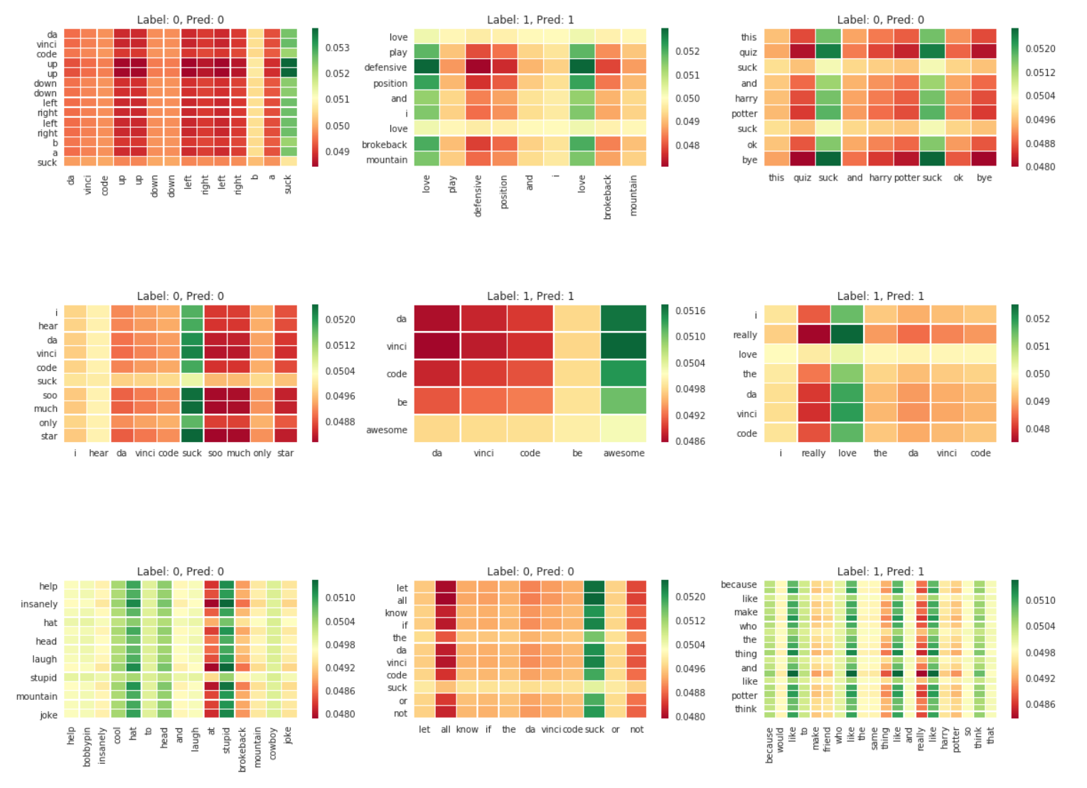
We can understand what tokens the algorithm pay attention to when it classifies the text. As is expected, sentiment words such as ‘love’, ‘awesome’, ‘stupid’, ‘suck’ got some spotlight during classification process.

Back to Posts

Sentiment Analysis - Self attention based on Relation Network